Dose-response curves (single drug)
Drugs are administered in specific doses, so the drug’s effect is measured per each dosage. After the experiments are done, you end up with measurements for each drug in the form: \((x,y)\), where \(x\) is the dosage and \(y=E \in [E_{min},E_{max}]\) the measured effect/viability/response (depending on which definition you use). You can plot these points to get the dose-response or dose-effect curve. Usually we assume that these curves are monotonous (always increasing or decreasing) though that may not always be true.3 There exist mathematical formulas that describe them, the most prominent of which is the 4-parameter log-logistic (4PL) model (Yadav et al. 2015):
\[\begin{equation} E = \frac{E_{min}+E_{max}\left(\frac{x}{m}\right)^\lambda}{1+\left(\frac{x}{m}\right)^\lambda} \tag{1.1} \end{equation}\]
Note that \(\lambda\) is the sigmoidicity of the curve and \(m\) is the dosage of the drug that produces half the maximum effect (also defined in various texts as \(EC_{50},IC_{50}\)). For \(E_{min}=0\), this equation is called Hill’s equation. A kind of derivative equation from (1.1) was proposed by (Chou and Talalay 1984) and it’s called the median effect equation:4
\[\begin{equation} \frac{f_a}{f_u} = \frac{y-E_{min}}{E_{max}-y}=\left(\frac{x}{m}\right)^\lambda \tag{1.2} \end{equation}\]
Where \(f_a+f_u=1\). The goal when plotting this function is to find a way to measure the \(m,\lambda\) parameters. (Chou and Talalay 1984) proposed to rewrite equation (1.2) as (generating what they called the medial effect plot):
\[\begin{equation} log\left(\frac{f_a}{1-f_a}\right)=\lambda\log x-\lambda\log m \tag{1.3} \end{equation}\]
Where we can easily compute the \(m,\lambda\) parameters (one is the slope, the other can be found where the plot cuts the \(x\)-axis: \(y=log\left(\frac{f_a}{1-f_a}\right)=0\)). Using Equation (1.1) and setting \(E_{max}=1,E_{min}=0\) and as \(x\) the \(x/m\), we can see how the sigmoidicity parameter \(\lambda\) affects the shape of the curve:
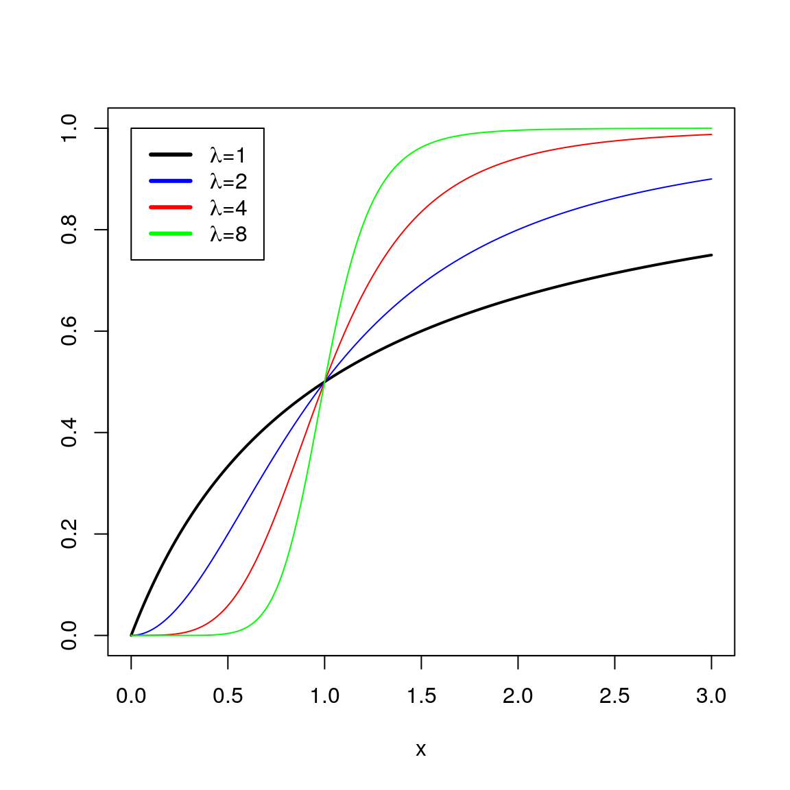
Figure 1.1: Hill’s equation for different values of the slope parameter λ
Note that for \(\lambda=1\) the shape is a hyperbole.
Also, using equation (1.2), we can compute any dose \(x\) as:
\[\begin{equation} x = m\left(\frac{f_a}{f_u}\right)^{1/\lambda} = m\left(\frac{y-E_{min}}{E_{max}-y}\right)^{1/\lambda} \tag{1.4} \end{equation}\]
Experiments, experiments… I have seen dose-response curves that have outliers: so while the curve was monotonously descreasing, you have one point that creates a little step hill before ultimately going down!↩︎
This equation fits to the expectation of the mass-action law principle that dictates many biological processes such as cell growth or ligand-binding interactions – it’s the unified theory for the Michaelis-Menten equation, Hill’s equation, Henderson-Hasselbalch equation and Scatchard equation (Chou 2006)↩︎