── Attaching core tidyverse packages ──────────────────────── tidyverse 2.0.0 ──
✔ dplyr     1.1.4     ✔ readr     2.1.5
✔ forcats   1.0.0     ✔ stringr   1.5.1
✔ ggplot2   3.5.1     ✔ tibble    3.2.1
✔ lubridate 1.9.3     ✔ tidyr     1.3.1
✔ purrr     1.0.2
── Conflicts ────────────────────────────────────────── tidyverse_conflicts() ──
✖ dplyr::filter() masks stats::filter()
✖ dplyr::lag()    masks stats::lag()
ℹ Use the conflicted package (<http://conflicted.r-lib.org/>) to force all conflicts to become errors
In the period 1962-77 a total of \(205\) patients with malignant melanoma (cancer of the skin) were operated at Odense University hospital in Denmark. A number of covariates were recorded at operation, and the patients were followed up until death or censoring at the end of the study at December 31, 1977. We will study death from malignant melanoma considering death from other causes as censorings. (Source: Andersen, Borgan, Gill & Keiding, Springer, 1993.)
Straight slope => constant hazard independent of gender
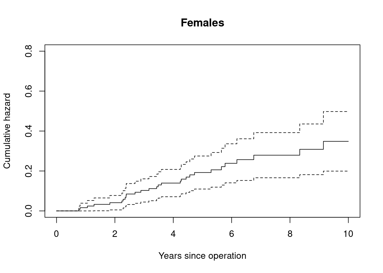
Make Nelson-Aalen plots for patients with ulceration present and absent and interpret the plots. (Ulceration is “present” if the surface of the tumor viewed in a microscope show signs of ulcers and “absent” otherwise.)
In this exercise, we will use the Kaplan-Meier estimator and the log-rank test to study survival for the melanoma patients.
We will consider Kaplan-Meier estimates for the mortality from malignant melanoma treating death from other causes as censoring.
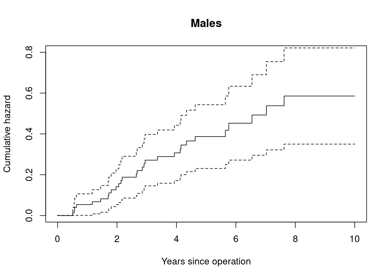
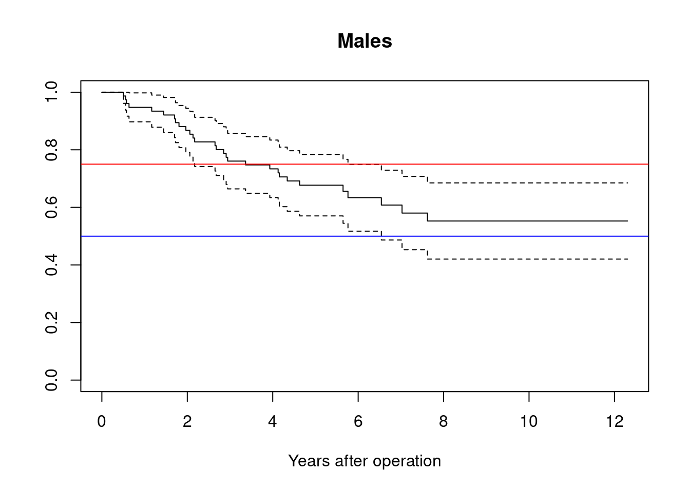
We may compute and plot the Kaplan-Meier estimate of the survival distribution for male patients by the commands (you need to load the survival-library)
fit.m=survfit(Surv(lifetime,status==1)~1,data=melanoma, subset=(sex==2), conf.type="plain")plot(fit.m, mark.time=FALSE, xlab="Years after operation", main ="Males")abline(h =0.75, col="red")abline(h =0.5, col="blue")
To obtain a summary of the results, you may give the command:
Perform these commands and interpret the Kaplan-Meier plot. Determine the lower quartile of the survival distribution for males with 95% confidence limits using the output from the summary-command. (Note that the lower quartile corresponds to 75% survival probability.)
Look at the first time the Survival probability falls below \(75\%\)
We may obtain the quartiles of the survival distribution for males by the command
quantile(fit.m)
$quantile
      25       50       75
3.364384       NA       NA

$lower
      25       50       75
2.172603 6.542466       NA

$upper
      25       50       75
5.761644       NA       NA
Perform this command and compare with the result you obtained in a).
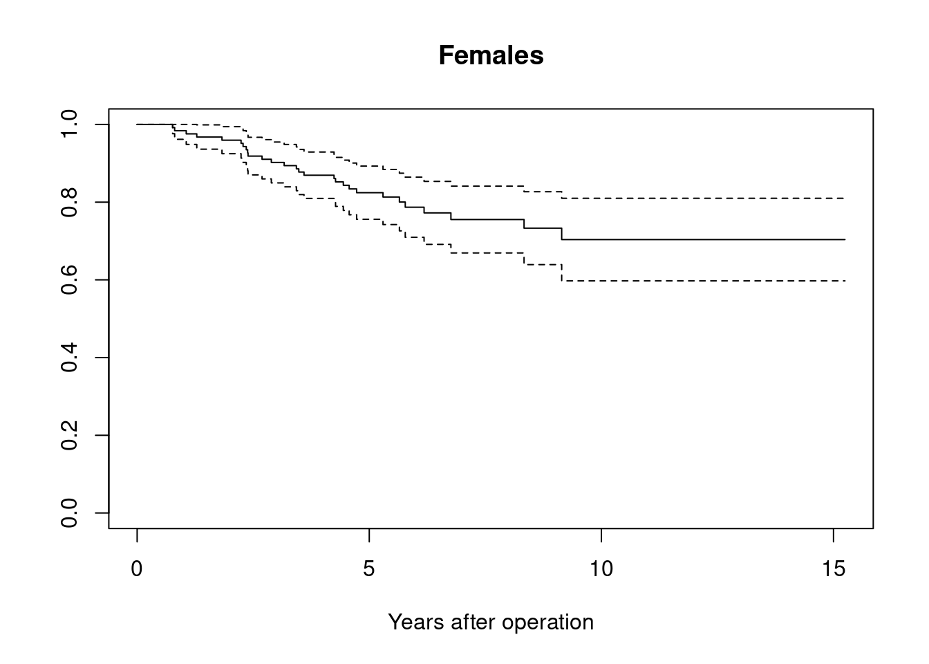
Make a Kaplan-Meier plot for females, and determine the lower quartile for females with 95% confidence limits (if possible). Compare with the results for males.
fit.f=survfit(Surv(lifetime,status==1)~1,data=melanoma, subset=(sex==1), conf.type="plain")plot(fit.f, mark.time=FALSE, xlab="Years after operation", main ="Females")
quantile(fit.f)
$quantile
      25       50       75
8.334247       NA       NA

$lower
     25      50      75
5.29589      NA      NA

$upper
25 50 75
NA NA NA
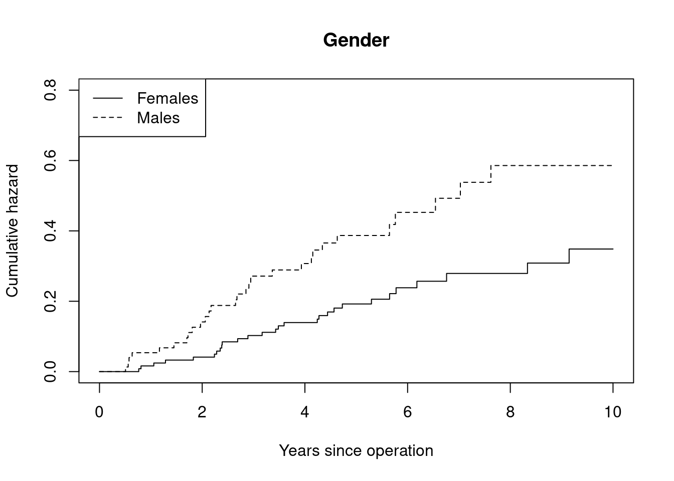
Use the log-rank test to test the null hypothesis that males and females have the same mortality from malignant melanoma:
Call:
survdiff(formula = Surv(lifetime, status == 1) ~ sex, data = melanoma)

        N Observed Expected (O-E)^2/E (O-E)^2/V
sex=1 126       28     37.1      2.25      6.47
sex=2  79       29     19.9      4.21      6.47

 Chisq= 6.5  on 1 degrees of freedom, p= 0.01
What may you conclude from the test?
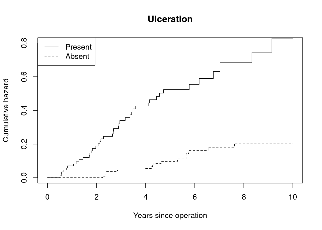
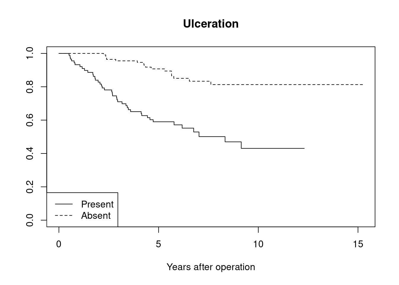
Make Kaplan-Meier plots for patients with ulceration present and absent and interpret the results. Is it possible to estimate the lower quartile for both ulceration groups? Estimate the lower quartile with confidence limits if possible. Is there a significant difference in cancer mortality for patients with ulceration present and absent?
plot(surv.ulcer, mark.time=FALSE, lty =1:2, xlab="Years after operation", main ="Ulceration")legend("bottomleft", c("Present","Absent"), lty=1:2)
quantile(surv.ulcer)
$quantile
                            25       50 75
strata(ulcer)=ulcer=1 2.690411 8.334247 NA
strata(ulcer)=ulcer=2       NA       NA NA

$lower
                            25       50 75
strata(ulcer)=ulcer=1 2.060274 4.728767 NA
strata(ulcer)=ulcer=2 7.621918       NA NA

$upper
                            25 50 75
strata(ulcer)=ulcer=1 4.126027 NA NA
strata(ulcer)=ulcer=2       NA NA NA
# NO STRATA IN THE FORMULA NEEDED!survdiff(formula =Surv(lifetime, status ==1) ~ ulcer, data = melanoma)
Call:
survdiff(formula = Surv(lifetime, status == 1) ~ ulcer, data = melanoma)

          N Observed Expected (O-E)^2/E (O-E)^2/V
ulcer=1  90       41     21.2      18.5      29.6
ulcer=2 115       16     35.8      10.9      29.6

 Chisq= 29.6  on 1 degrees of freedom, p= 5e-08
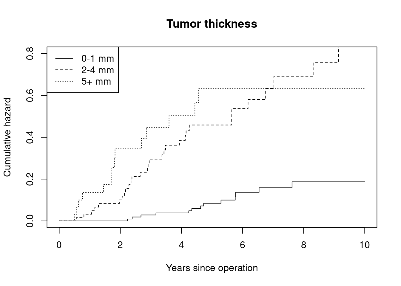
Make Kaplan-Meier plots for the three thickness groups 0-1 mm, 2-4 mm, 5+ mm and interpret the plots. Estimate the lower quartile with confidence limits if possible. Is there a significant difference in cancer mortality between the three thickness groups?