Multi-state models

library(survival)
library(mstate)
library(tibble)
library(dplyr)


Attaching package: 'dplyr'

The following objects are masked from 'package:stats':

    filter, lag

The following objects are masked from 'package:base':

    intersect, setdiff, setequal, union

In this exercise, we will see how we may find the Nelson-Aalen estimates for the cumulative transition intensities and the Aalen-Johansen estimates for the transition probabilities in a Markov illness-death model. To this end, we will use the bone marrow transplantation data described in example 1.13 in the ABG-book and used for illustration in example 3.16. To read the data into R you may give the command:

bonemarrow = read.table("https://www.med.uio.no/imb/english/research/centres/ocbe/courses/imb9335/bone-marrow.txt",header=T) %>% as_tibble()
bonemarrow %>% select(T2, DF, TP, P)

# A tibble: 137 × 4
      T2    DF    TP     P
   <int> <int> <dbl> <int>
 1  2081     0    13     1
 2  1602     0    18     1
 3  1496     0    12     1
 4  1462     0    13     1
 5  1433     0    12     1
 6  1377     0    12     1
 7  1330     0    17     1
 8   996     0    12     1
 9   226     0    10     1
10  1199     0    29     1
# ℹ 127 more rows

Bone marrow transplantation data:

g => Disease Group (1: ALL, 2: AML Low Risk, 3: AML High Risk)
T1 => Time To Death Or On Study Time
T2 => Disease Free Survival Time (Time To Relapse, Death Or End Of Study)
D => Death Indicator (1: Dead, 0: Alive)
R => Relapse Indicator (1: Relapsed, 0: Disease Free)
DF => Disease Free Survival Indicator (1: Dead Or Relapsed, 0: Alive Disease Free)
TA => Time To Acute Graft-Versus-Host Disease
A => Acute GVHD Indicator (1: Developed Acute GVHD, 0: Never Developed Acute GVHD)
TC => Time To Chronic Graft-Versus-Host Disease
C => Chronic GVHD Indicator (1-Developed Chronic GVHD, 0:Never Developed Chronic GVHD)
TP => Time To Return of Platelets to Normal Levels
P => Platelet Recovery Indicator (1: Platelets Returned To Normal, 0-Platelets Never Returned to Normal)
Z1 => Patient Age In Years
Z2 => Donor Age In Years
Z3 => Patient Sex (1-Male, 0-Female)
Z4 => Donor Sex (1: Male, 0: Female)
Z5 => Patient CMV Status (1: CMV Positive, 0: CMV Negative)
Z6 => Donor CMV Status (1: CMV Positive, 0: CMV Negative)
Z7 => Waiting Time to Transplant In Days
Z8 => FAB (1: FAB Grade 4 Or 5 and AML, 0: Otherwise)
Z9 => Hospital (1:The Ohio State University, 2: Alferd , 3: St. Vincent, 4: Hahnemann)
Z10 => MTX Used as a Graft-Versus-Host- Prophylactic (1:Yes, 0:No)

The data contain information for \(137\) patients with acute leukemia who had a bone marrow transplantation. The patients were followed for a maximum of seven years, and times to relapse and death were recorded. It was also recorded if and when the platelet count of a patient returned to a self-sustaining level. The possible events for a patient may be described by an illness-death model without recovery with the three states “transplanted”, “platelet recovered”, and “relapsed or dead”. A patient starts out in state “transplanted” at time zero when he/she gets the bone marrow transplant. If the platelets recover, the patient moves to state “platelet recovered”, and if he/she then relapses or dies, the patient moves on to state “relapsed or dead”. If the patient relapses or dies without the platelets returning to a normal level, he moves directly from state “transplanted” to state “relapsed or dead”.

To find the Nelson-Aalen estimates and the empirical transition probabilities (i.e. Aalen-Johansen estimates) we will use the mstate package so this has to be installed and loaded.

We start out by defining the states and the possible transitions between them. This is achieved by the command:

tmat = transMat(x = list(c(2,3),c(3),c()), names = c("transplanted","recovered","relapsed.dead"))
tmat

               to
from            transplanted recovered relapsed.dead
  transplanted            NA         1             2
  recovered               NA        NA             3
  relapsed.dead           NA        NA            NA

To perform the estimation, we need to convert the data-frame to a long format, where there are 2-3 lines for each patient:

bonemarrow.long = msprep(time=c(NA,"TP","T2"), status=c(NA,"P","DF"),data=bonemarrow,trans=tmat)
bonemarrow.long %>% as_tibble()

# A tibble: 394 × 8
      id  from    to trans Tstart Tstop  time status
   <dbl> <dbl> <dbl> <dbl>  <dbl> <dbl> <dbl>  <dbl>
 1     1     1     2     1      0    13    13      1
 2     1     1     3     2      0    13    13      0
 3     1     2     3     3     13  2081  2068      0
 4     2     1     2     1      0    18    18      1
 5     2     1     3     2      0    18    18      0
 6     2     2     3     3     18  1602  1584      0
 7     3     1     2     1      0    12    12      1
 8     3     1     3     2      0    12    12      0
 9     3     2     3     3     12  1496  1484      0
10     4     1     2     1      0    13    13      1
# ℹ 384 more rows

# example
bonemarrow %>% as_tibble() %>% filter(T2 == 383)

# A tibble: 1 × 22
      g    T1    T2     D     R    DF    TA     A    TC     C    TP     P    Z1
  <int> <int> <int> <int> <int> <int> <int> <int> <int> <int> <dbl> <int> <int>
1     1   417   383     1     1     1   417     0   417     0    16     1    15
# ℹ 9 more variables: Z2 <int>, Z3 <int>, Z4 <int>, Z5 <int>, Z6 <int>,
#   Z7 <int>, Z8 <int>, Z9 <int>, Z10 <int>

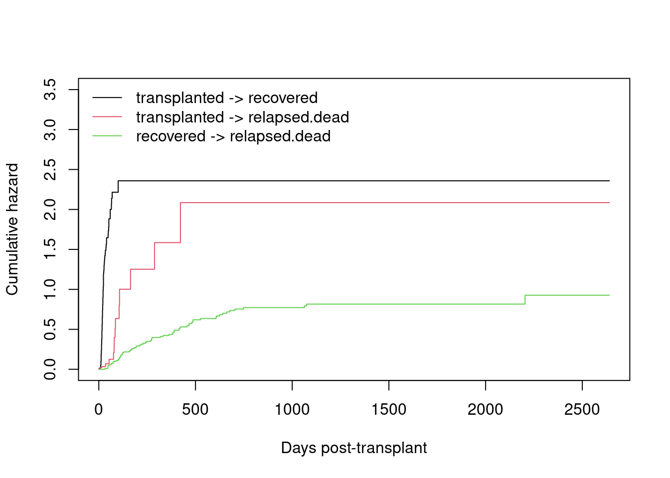
Then we fit a stratified Cox-model with no covariates (stratifying on the type of transition), extract the Nelson-Aalen estimates for the cumulative transition intensities and make a plot of these:

cox.bm=coxph(Surv(Tstart,Tstop,status)~strata(trans),data=bonemarrow.long, method="breslow")
haz.bm=msfit(cox.bm,trans=tmat)

plot(haz.bm,xlab="Days post-transplant",xlim=c(0,1000),ylim=c(0,3.5))

To find the Aalen-Johansen estimates of the transition probabilities, we give the command:

prob.bm = probtrans(haz.bm,predt=0)

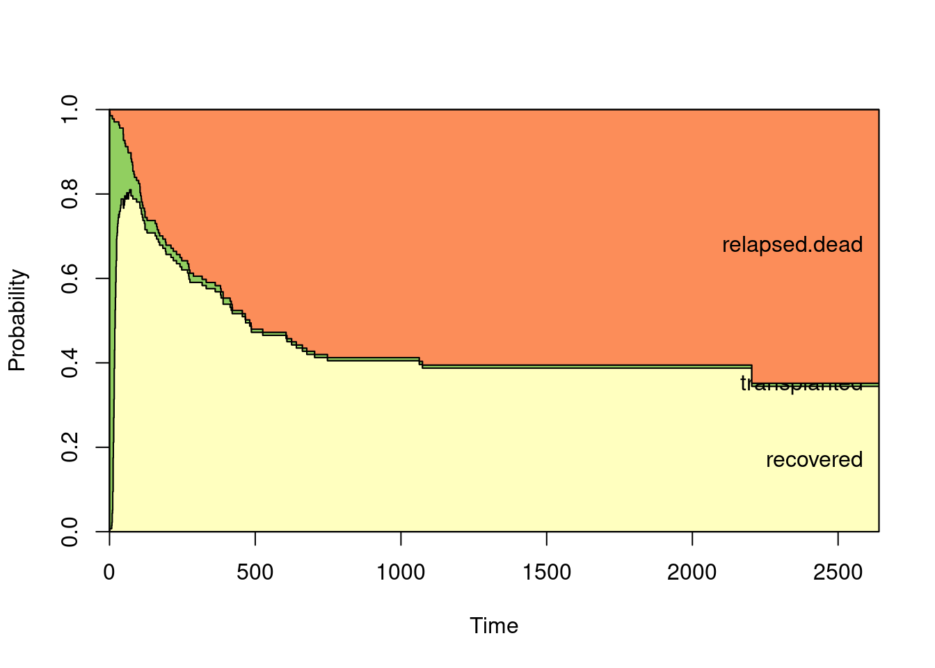
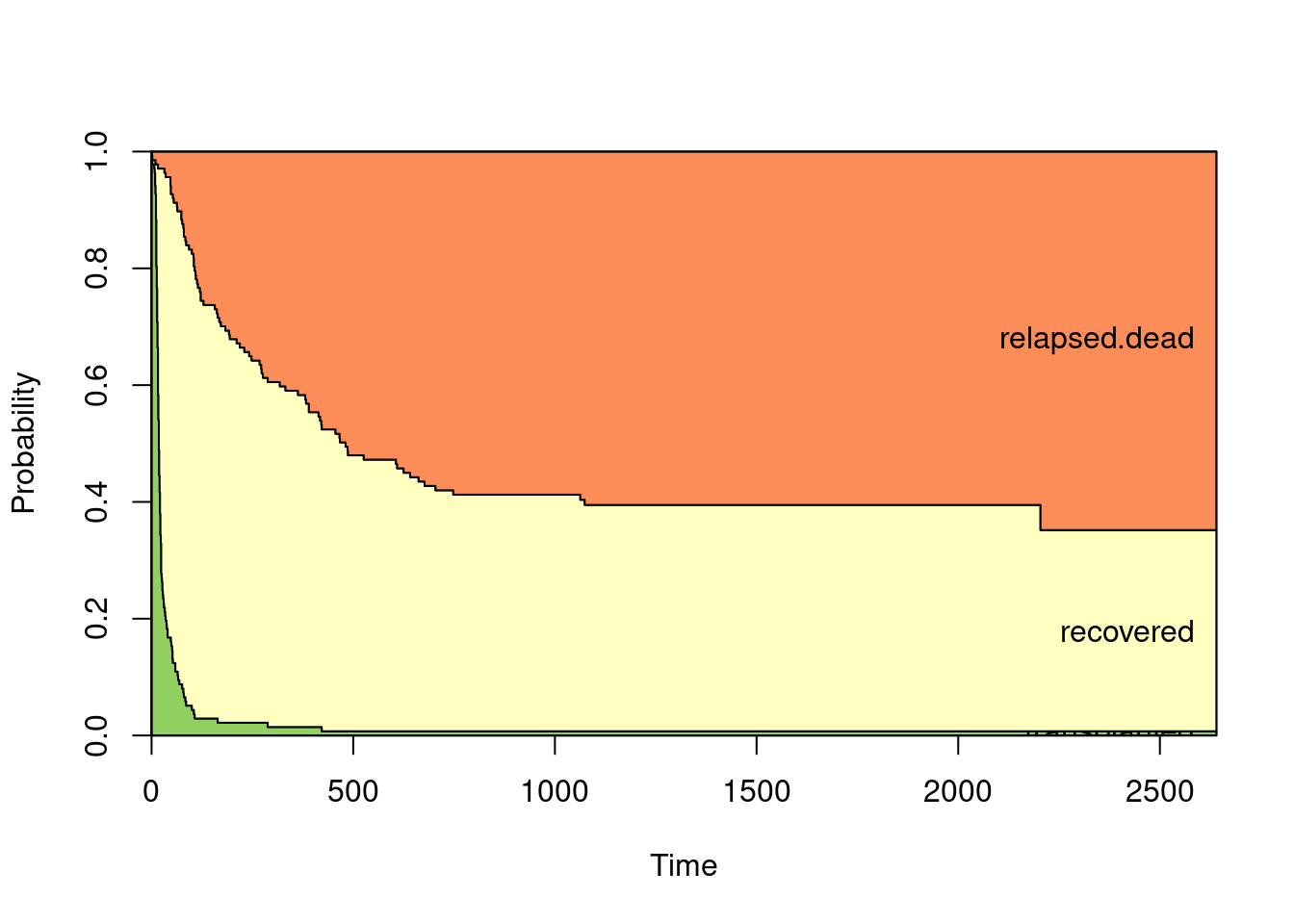
We may extract the empirical transition probabilities from state “transplanted” (state 1) by the command prob.bm[[1]], and similarly we obtain the empirical transition probabilities from state “recovered” (state 2) by prob.bm[[2]].

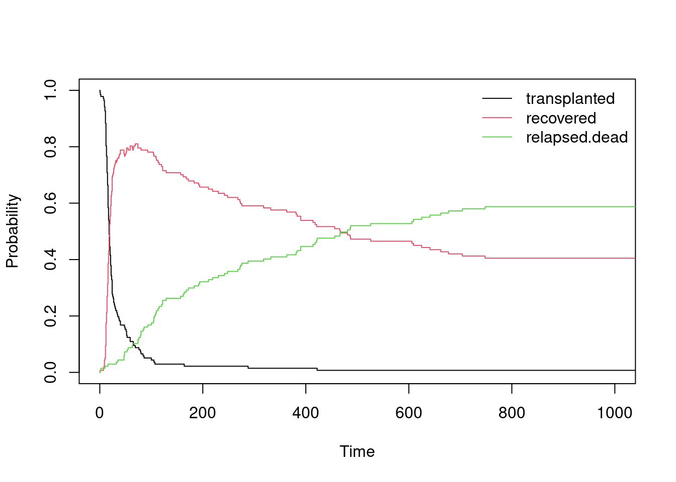
The transition probabilities may be plotted in a stacked manner or as separate estimates by the commands:

plot(prob.bm,type="filled",ord=c(2,1,3))

plot(prob.bm,type="filled")

Probability of being in each state:

plot(prob.bm,type="single",xlim=c(0,1000),col=1:3)

Perform the commands given above. Make sure that you understand what each of the commands and plots give you, and compare the results with those of example 3.16 in the ABG-book.
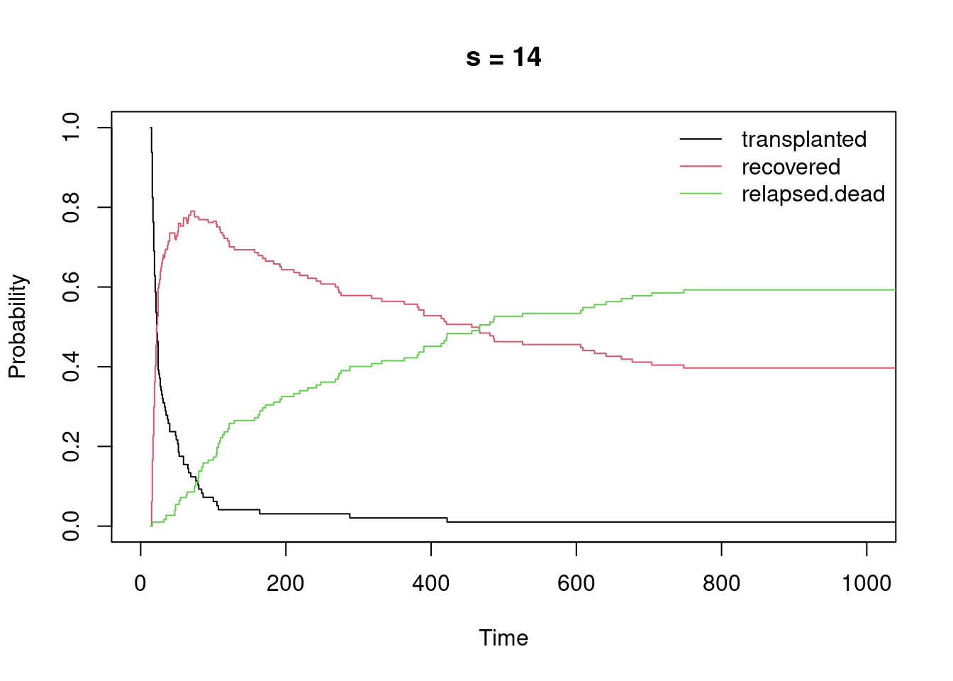
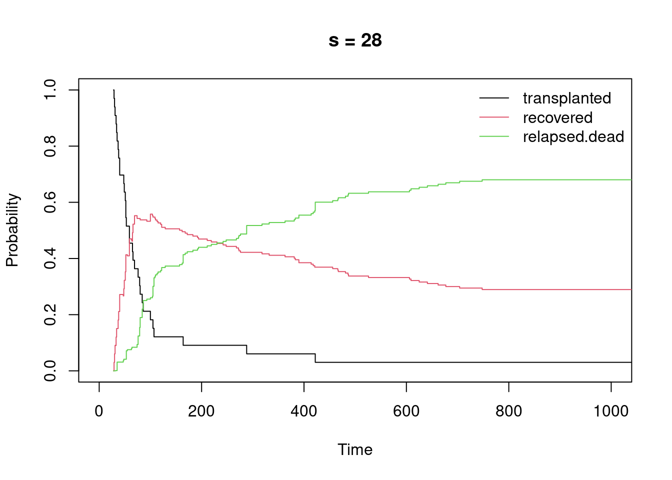
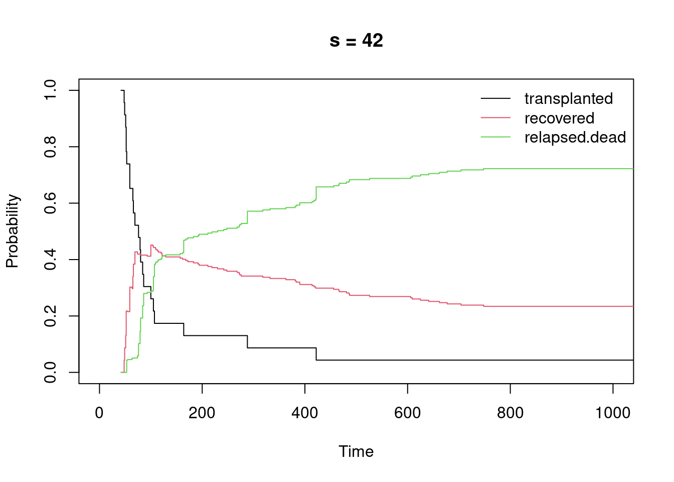
Above we used the probtrans command with the option predt=0. This gives transition probabilities from time s = 0 to time t. Also compute and plot the transition probabilities for \(s = 14, 28\) and \(42\). What can you learn from these plots?

prob.bm.14 = probtrans(haz.bm,predt=14)
plot(prob.bm.14, type = "single", xlim = c(0,1000), col = 1:3, main = 's = 14')

prob.bm.28 = probtrans(haz.bm, predt = 28)
plot(prob.bm.28, type = "single", xlim = c(0,1000), col = 1:3, main = 's = 28')

prob.bm.42 = probtrans(haz.bm,predt=42)
plot(prob.bm.42, type = "single", xlim = c(0,1000), col = 1:3, main = 's = 42')

What if I start from state 2?

plot(prob.bm.14, from = 2, type = "single", xlim = c(0,1000), col = 1:3, main = 's = 14 from 2nd Recovery state')

Reference:

Klein, JP and Moeschberger, ML (2003) Survival analysis. Techniques for Censored and Truncated Data (2nd edition). Springer-Verlag, New York.